Inflating away your pension

As a result of their negotitations on the future of UK university pensions, which I have written about previously, the University and College Union (UCU) and employers represented by Universities UK (UUK) announced an agreement on 12 March 2018. The main points of the agreement are:

• Change the accrual rate from 1/75 to 1/85 per year of service
• Increase employee contributions from 8% to 8.7%
• Cap the increases of accrued pensions at CPI up to 2.5% p.a.

While the effect of the first two changes on the value of future pensions is relatively straightforward to analyse, the effect of the inflation cap is not obvious. In the first attempt to model the effect of this proposal that I am aware of, Richard Wilkinson finds a substantial real-terms loss to pensions if inflation history exactly repeats the last 40 years. The figure below shows the annual inflation rate since 1976, the year after the University Superannuation Scheme (USS) was founded, and the proposed inflation cap at 2.5%.

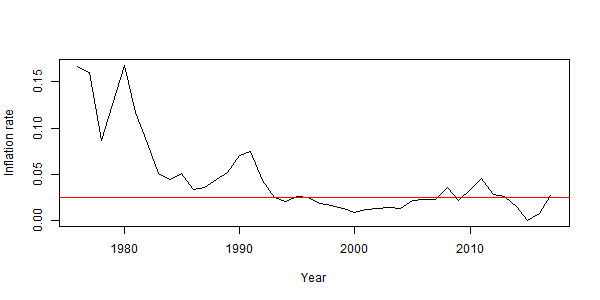
If inflation runs at a rate higher than the 2.5% cap, accrued pensions will increase by 2.5% per year, causing a loss in value of these accrued pensions in real terms. With consumer price inflation (CPI) at 2.7% in 2017, some might ask what the effect of the inflation cap will be on their expected pension. More precisely, what will be the effect of the inflation cap on the value of newly accrued pension rights?

We can find an answer empirically by simulating possible future paths of inflation. It may be reasonable to assume that future inflation will be similar to past inflation in the period 1976-2017. Suppose that future rates of inflation will be the same as inflation from the inception of the USS until 2017 with equal likelihood for each annual rate. We can then simulate future outcomes by drawing random samples from these years, each with a length equal to the number of years left before retirement. For this example, we will assume that retirement is still 20 years away. If we draw a year in which inflation was higher than 2.5%, we cap it at 2.5%. The pension value for each sample is then obtained as the product of all 20 inflation values (plus one).

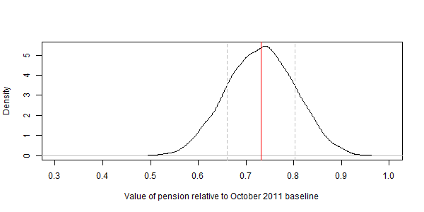
The value of accrued pensions under the new inflation cap rule can then be expressed relative to either full inflation adjustment (i.e., no inflation cap) or the current inflaton adjustment regime under the October 2011 rule (i.e., full adjustmen up to 5%, then 5% + one half of increase above 5% until 15%, capped at 10% p.a., see USS factsheet).

Simulation results show that pensions under the proposed 2.5% inflation cap are worth about 73% of pensions under the current adjustment rule. In other words, the proposed inflation cap reduces pensions by about 27% compared with current USS rules, in addition to the value reduction through increased contributions and a lower accrual rate. The distribution of pension values relative to the October 2011 inflation rule is shown below. This kernel density estimate of the distribution is based on 10,000 draws of 20 annual inflation rates each. Likely outcomes within one standard deviation of the mean are between 66% and 80% of current pensions.

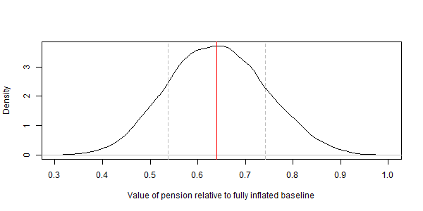
For completeness, the figure below shows pension values if outcomes using the proposed inflation cap are compared with outcomes using full inflation adjustment. If accrued pensions were adjusted fully in line with consumer prices, pensions under the proposed new regime would be worth 64% of this baseline outcome on average.

How likely is history to repeat itself?

Short answer: we don’t know. Mike Otsuka, who has modelled the USS proposal in late 2017, has pointed out in his posts that the high-inflation period of the late 1970s and early 1980s may be unlikely to repeat because in 1992 the Bank of England adopted the policy of inflation targeting with a target of 2%. Ian Sudbery has done some calculations and finds results in line with my results shown above. Readers are invited to use my code and experiment with different time periods.

The likelihood of history repeating itself ultimately depends on the credibility of central bank policy. The Bank of England may currently subscribe to a 2% p.a. inflation target, but its motivation and ability to commit to this policy for decades to come may be questioned. There is evidence that the Bank of England may tolerate an inflation overshoot. Even the most recent data suggests that the inflation cap of 2.5% would have been binding in December 2017 when CPI was at 3% year-on-year (and RPI was at 4.1%). If an inflation cap is set near the targeted inflation rate, there will be periods in which inflation overshoots the cap, which will result in real losses to pensions. BoE policy with regard to the magnitude of a desirable or tolerable inflation overshoot (e.g., to compensate for a previous undershoot) is subject to an ongoing debate and far from fixed.

In a recent interview with former Federal Reserve chairman Ben Bernanke, his successor Janet Yellen admitted that some of the Fed’s policies “require a degree of commitment that’s, I think, difficult to achieve given the governance arrangements that most central banks have. It’s not impossible for committees to make sort of long-term commitments with some credibly.” As a result, market participants do not see central bank policy as fixed either. If the inflation target can slip in periods of lower inflation, it is conceivable that it may shift higher in periods of higher inflation due to a drop in the exchange rate and imported inflation or domestic fiscal policy aimed at fending off the next recession.

Update: Effect on today’s contribution vs all future contributions

While the analysis above tracks the fate of a single pound that is added to the pension pot today, we could also ask what would happen to all future or past pension contributions. Unfortunately, the 12th March proposal is not very clear about whether the inflation cap would apply to benefits accrued in the past (it says the inflation indexing “includes revaluation of the salary threshold, revaluation of accrual of benefits (pre-retirement) and guaranteed pension increases”). So let’s assume the inflation cap would only apply to future contributions.

To find the future value of all future pensions, we need to change the expression “prod(drawcap+1)/prod(draw+1)” in the code below. A solution that assumes constant contributions was suggested to me by Jon Forster and involves replacing “prod(drawcap+1)” with “sum(cumprod(drawcap+1))”. The denominator would be adjusted appropriately, keeping the contributions constant or using the same salary growth rates as in the numerator. If salaries increase in line with capped inflation, we have

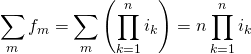
for the sum of future values of all contributions, where f_m is the future value of a contribution made in year m, i_k is the (potentially capped) inflation rate in year k, and n is the number of years until retirement.

If the assumption that salaries increase in line with pensions is relaxed, we have

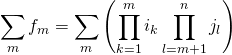
where i_k is the (potentially capped) rate of salary growth and j_l is the (potentially capped) rate of growth of accrued benefits. Intuitively, salaries will increase by i_k from today until the contribution is made. From this point in time on, contributions (i.e., accrued benefits) will be revalued at the rate j_l until retirement.

Would this alternative calculation method make a difference? Probably, but this not only depends on the inflation cap (and inflation rate) but also on assumptions about future salary growth. In addition, given the history of USS rule changes, it seems prudent to use a relatively short time horizon. The annual economic effect of an inflation cap on future contributions will be the same as its effect on this year’s contribution, which is an expected real interest rate penalty. The longer this negative rate is applied, the larger its effect will be, which means that future contributions will suffer a smaller real loss simply because the annual penalty is not applied as often.

Data and code for replication

Inflation data are from the Office for National Statistics. I have used CPI data (series D7G7) for the years 1989 to 2017 and RPI (ex mortgage & council tax, series DQAD) for the period from 1976 to 1988 for lack of a CPI times series for this period. RPI has been reported to be slightly higher than CPI on average, but excluding the high-inflation year of 1975 (when the USS was founded) should reduce this effect. The dataset is available here.

The above figures were created in R using the code below.

## Set up data 
dat<-read.csv("inflation_UK.csv",header=T,sep=",") 
dat<-dat[-1,] #keep all values from 1976 

## History of inflation 
plot(dat[,c("year","i")],ylab="Inflation rate",xlab="Year",type="l") 
abline(h=0.025,col="red") 

## How far away is your pension (in years)? 
futureyears<-20 

## Simulate the future relative to full inflation adjustment 
res<-as.numeric() ## empty vector for results 
for(t in 1:10000){ 
  draw<-sample(dat$i,size=futureyears,replace=T) 
  drawcap<-ifelse(draw>0.025,0.025,draw) 
  res<-c(res,prod(drawcap+1)/prod(draw+1)) 
} 

## Show results 
lot(density(res),xlim=c(0.3,1),main="",xlab="Value of pension relative to fully inflated baseline") 
abline(v=mean(res),col="red") 
abline(v=c(mean(res)+sd(res),mean(res)-sd(res)),col="grey",lty=2) 

## Simulate the future relative to October 2011 inflation adjustment 
res<-as.numeric() ## empty vector for results 
for(t in 1:10000){ 
  draw<-sample(dat$i,size=futureyears,replace=T) 
  drawoldcap<-ifelse(draw>0.05,ifelse(draw<0.15,0.05+0.5*(draw-0.05),0.1),draw) 
  drawnewcap<-ifelse(draw>0.025,0.025,draw) 
  res<-c(res,prod(drawnewcap+1)/prod(drawoldcap+1)) 
} 

## Show results 
plot(density(res),xlim=c(0.3,1),main="",xlab="Value of pension relative to October 2011 baseline") 
abline(v=mean(res),col="red") 
abline(v=c(mean(res)+sd(res),mean(res)-sd(res)),col="grey",lty=2)